Where v1 left off
The first version of Nebula built its whole inverted index in memory, from scratch, on every run. That was fine for a few hundred books, but indexing ~1,000 books took anywhere from 5 to 30 minutes and the index lived and died with the process. The two "what's next" items at the end of v1 became the two goals of v2:
- Scale up. Make the index persistent so it can grow toward the full ~80,000-book Gutenberg catalog without ever needing to fit in RAM.
- Rank better. Implement BM25 and measure it against TF‑IDF and its TF-only / IDF-only ablations on the same precision/recall benchmarks.
Going in, I wrote down three hypotheses: BM25 would improve precision and recall, partitioning would improve query time, and index size would scale linearly with corpus size.
Pipeline
Indexing now happens in waves of ~1,000 books, each one appended to partitions on disk. Queries only ever open the partitions their terms hash to:
Scaling the hardware first
The first attempt at 10k documents overwhelmed my laptop's hard drive. The Gutenberg corpus is roughly 100 GB of plain text at 80k books, so the books themselves moved onto a NAS mounted over a local network, freeing local disk for the index — which is the thing that actually needs to be fast to read.
Before going further, I measured how big the index gets as the corpus grows:
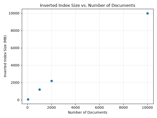
That hypothesis held up: the index grows linearly, at about 1 GB per 1,000 books. That's a clean rule of thumb, and it's also the bad news — the full catalog would be an ~80 GB index. Loading that into memory isn't an option, so the index had to be split up and persisted.
A persistent, partitioned index
A PartitionedInvertedIndex is just a list of ordinary v1-style
InvertedIndex objects. Every word is routed to one of them by a small polynomial
string hash, so a given word always lands in the same partition, in every wave:
Each partition is persisted as a flat, append-only TSV file (1of500.tsv,
2of500.tsv, …), one posting per line. Appending is what makes waves work: a new batch
of books builds small temporary partitions in memory, then each one is appended onto its
matching file on disk.
Alongside the partitions sits a manifest — one (dataset, book, length)
row per indexed book. It's small enough to always live in memory, where it does two separate
jobs: it stops a book from being indexed twice if a wave is re-run, and it holds every book's word
count, which TF and BM25 both need. Two different purposes in memory, but convenient to persist
together. The full index itself is never entirely in memory at any point.
Query time vs. number of partitions
At query time, each query term is hashed to find its partition, and only those files are read.
The benchmark: a 10k-book (~10 GB) index, the 5-term query
treasure voyage adventure pirates swords, run 10 times per configuration, with mean
run time to execute the search query against the partitioned index as the benchmark measurement.
First, a slow start
The very first run with 5 partitions took 534 seconds — almost nine minutes for one query. My first guess was that the manifest was being reloaded every time a partition was read, since I was reusing the full loader. Fixing that changed nothing (536 s). The real problem was that loading a partition rebuilt its entire index in memory just to look up a handful of words. A loader that skips irrelevant line fixed the issue:
That brought the 5-partition query down to ~142 s. Then the real study began:
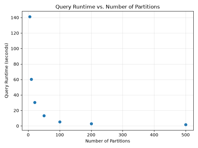
| Partitions | 5 | 10 | 20 | 50 | 100 | 200 | 500 |
|---|---|---|---|---|---|---|---|
| Mean query time | 141.3 s | 60.2 s | 30.3 s | 13.4 s | 5.3 s | 2.9 s | 1.6 s |
I expected a "V": more partitions means smaller files to scan, until the overhead of opening and closing lots of files takes over and query time climbs back up. With a single 5 word query, that behavior never manifested. Query time kept falling roughly in proportion to partition size all the way to 500 partitions, where a 5-term query takes about a second and a half — so I stopped there.
Even though the graph doesn't show it, but V shape behavoir still exists, but only with long queries. A stem$ wildcard can expand into dozens of terms via
the trie, and each term can hit a different partition. With enough terms, a query touches most
of the files and can take 30+ minutes. The CLI now warns and asks for confirmation when a
wildcard expands to more than a certain number of terms; capping query length at the UI is a quick fix that doesn't need more thought at least for now.
The trie, now with document frequency
I'm hoping to build not just a search engine, but a services that helps with understanding unstructured data. One of the key insights I had during v1 was how important document frequency is when understanding, which search terms are useful and which search terms will pull you into the weeds. Really crafting your search terms to search high value words is a good starting place. In v2 each node in the trie carries a
df counter, and a new /trie <stem> command lists every indexed word
under a stem along with its count — handy for checking how common a term is before querying it.
At 10k books the trie is large but still fits in memory, so it's pickled to disk and loaded at
startup. __slots__ drops each node's per-instance __dict__, which adds up
across millions of nodes, and it seemed to speed up loading and saving the trie.
BM25
During my literature reivew of information retrieval algorithms, I started with what we will call naive TF-IDF. This represents most basic implementation of combining the term frequency metric (TF) of "A Statistical Approach to Mechanized Encoding and Searching of Literary Information" (1957-Luhn) with the weighting by specificy metric now called inverse document frequency metric (IDF) of "A statistical interpretation of term specificity and its application in retrieval" by Karen Spärck Jones (1972-Jones). Naive TF-IDF just calculates the two metrics individually and multiplies them together. For Nebula_v1, that was the calculation.
By the 90s, there were many different types of TF-IDF metrics, and what is now called BM25 or Okapi BM25 seems to be the most referenced, so that is what was implemented in Nebula_v2. The three papers that seemed to most clearly explain this algorithm to the world are:
- "Okapi at TREC" (1993-Robertson). The first BM algorithm/formula called "the F4 formula". Reference explains the full IR system.
- "Simple, proven approaches to text retrieval" (1994-Robertson). The first reference to the formula as BM25, see eq. (2).
- "Okapi at TREC-3" (1995-Robertson). This paper provides a full evolution of the formula from BM1 through BM11 and BM15, and finally, to BM25.
Naive TF‑IDF has two weaknesses. TF grows without limit, so a book that says "voyage" 400 times scores twice as high as one that says it 200 times, even though both are clearly about voyages. And dividing by document length is a blunt way to correct for long books. BM25 changes both pieces:
- Saturation (
k): each extra occurrence of a term is worth less than the last, so one term can't drown out the rest of the query. - Length normalization (
b): a book is compared to the average book length, and only partially, instead of dividing raw counts by length. - Smoothed IDF: the
+0.5and+1keep the IDF from going negative or blowing up for very common or very rare terms.
The average document length is computed once from the manifest, so BM25 costs about the same as naive TF‑IDF at query time.
Precision & recall: BM25 vs. naive TF‑IDF
For relevance labels I used Gutenberg's own bookshelf metadata instead of tagging books by hand. Any book on the "Adventure" shelf counts as relevant to the adventure query, and any book on "Science Fiction" counts for the sci-fi query. The third query targets a single book: Treasure Island (book #120), but with some bad query terms mixed in to show the benefit of the BM25 calculation. Every query was scored four ways (BM25, TF‑IDF, TF only, IDF only) against the same 9,456-book index, measuring precision and recall in the top 20.
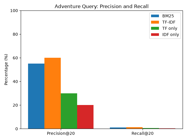
treasure voyage adventure pirates swords (957 relevant)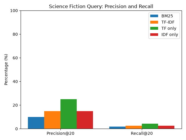
spaceship future technology alien planet (114 relevant)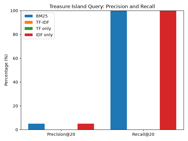
voyage yo-ho-ho travel weapons (1 relevant)| Precision@20 | Adventure | Sci-fi | Treasure Island (found #120?) |
|---|---|---|---|
| BM25 | 55% | 10% | yes |
| TF‑IDF | 60% | 15% | no |
| TF only | 30% | 25% | no |
| IDF only | 20% | 15% | yes |
Treasure Island is where BM25 shows its value
The Treasure Island query doesn't name the book. It describes it with three generic words and one
very specific one: yo-ho-ho. Naive TF‑IDF and TF-only both miss the book completely,
because the top 20 fills up with books that say "voyage" and "travel" over and over, and nothing
limits how much that repetition counts. BM25's saturation caps the reward for repeating common
words, which lets the rare, high-IDF term decide the ranking, and Treasure Island makes it
into the top 20.
IDF-only finds it too, for the same reason: it scores almost entirely on rarity. But on the broader adventure query IDF-only falls to 20% precision, while BM25 holds 55%, close to TF‑IDF's 60%.
The result isn't a clean sweep, though. The sci-fi query was hard for every method, and BM25 scored lowest on it at 10%. Words like "future" and "technology" are common across the whole corpus, and only 114 of ~9.5k books are on the sci-fi shelf. Bookshelf labels are also a rough measure of relevance: a book can be about pirates without being shelved as "Adventure." So the honest conclusion is that BM25 is the better general-purpose default, not that it beats TF‑IDF on every query. It's now the scorer the Nebula CLI uses.
What I took away
- Index size is linear at ~1 GB per 1,000 books, which makes planning storage for bigger corpora straightforward.
- Profile before you partition. The single biggest speedup (534 s → 142 s) came from skipping irrelevant lines in a loader, not from the architecture.
- Partitioning pays off more than I expected: 141 s → 1.6 s going from 5 to 500 partitions, with no sign yet of the file-I/O turnaround I predicted.
- BM25's saturation matters most on "needle" queries, where one rare term should beat a lot of repetition of common ones.
What's next: testing new data structures and algorihtms
From here, I've implemented what is commonly considered the best algorithms and practices for information retrieval. There are many optimizations available in the literature that deserve exploration. Two that I noticed that could be very helpful are inverted index compression and creating multiple inverted indexes, where the query parser chooses between the inverted indexes when deciding how to execute the query. For the next version, I'm not limiting myself to exploring these research directions, but leaving the option open if they help research goals. For the actual goals, I want to explore a few:
- Scaling the corpus to include 20k docs
- Indexing three word phrases rather than just single words
- Increase precision or recall by bundling documents
As the size of the corpus and index grow, the project should be subject to a few constraints. A document bundle cannot increase the size of the corpus by copying documents. This would result in an explosion in the size of the corpus. Additionally, indexing three word phrases will likely 3x the size of the inverted index, and because of the scaling study above, I know that would be about 60GB. Certain phrases that only include stopwords can be eliminated from this index like "is of the". Stopwords can be chosen algorithmically based on DF score (using the trie), rather than a hand-typed list.